I wrote the post
sp_execute_external_script and SQL Compute Context - I about how the SQL Server Compute Context (SQLCC) works with sp_execute_external_script (SPEES), as I wanted to correct some mistakes I did in the
Microsoft SQL Server R Services - sp_execute_external_script - III post. I initially thought one post would be enough, but quite soon I realised I was too optimistic, and at least one more post would be needed, if not more. So this is the first followup post about SPEES and SQLCC.
To see other posts (including this) in the series, go to sp_execute_external_script and SQL Server Compute Context.
One of the reasons for me realising that one post is not enough is that while I wrote and executed code for the first post, I noticed some fairly significant performance differences using SQLCC compared to not using SQLCC (SQLCC performed better :)). So that is part of what we look at in this post.
Recap
In quite a few posts about SQL Server Machine Learning Services we have discussed how, as part of the functionality in RevoScaleR, you can define where a workload executes. By default, it executes on your local machine, but you can also set it to execute in the context of somewhere else: Hadoop, Spark and also SQL Server. So, in essence, you can run some code on your development machine and have it execute in the environments mentioned above.
In the
Context - I post we saw that even when we executed from inside SQL Server, the compute context was the local context: RxLocalSeq. If we want to use the SQLCC we used RxInSqlServer and rxSetComputeContext:
|
|
Code Snippet 1: Set up SQL Server Compute Context
To setup the context we see in Code Snippet 1 how we use a connection string pointing to the SQL Server where we want to execute the code. In this case, it is the instance we are on.
NOTE: The connection string is for where we want to execute, not necessarily where the data we use resides.
We also see in Figure 1 how RxInSqlServer has the numTasks parameter for you to set the number of tasks (processes) to run for each computation. The parameter defines the maximum number of tasks SQL Server can use. SQL Server can, however, decide to start fewer processes. Finally in Figure 1 we call rxSetComputeContext which ensures that any code with functions that support SQLCC, executes under the compute context.
In the Context - I post, we saw how when we execute inside of SQL Server via SPEES we by default run in the local context and only by setting the context as in Code Snippet 1 we can execute in SQLCC.
An interesting observation when we set the numTasks parameter to a value greater than 1 is that when we run the code, we run it hosted in an mpiexec.exe process:
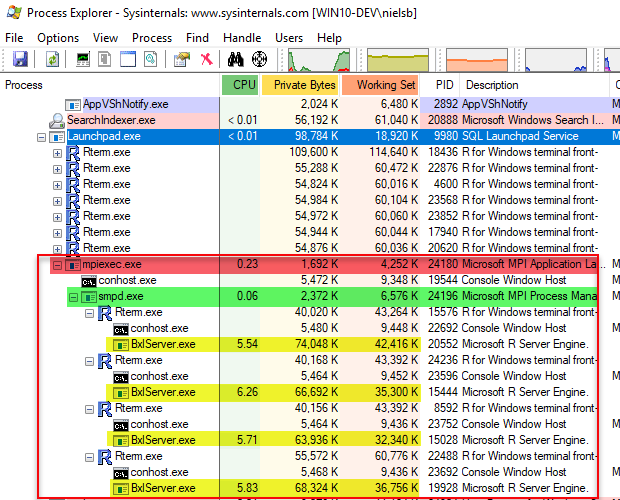
Figure 1: Parallel Execution in Compute Context
In Figure 1 we now see not only the “usual” RTerm and BxlServer.exe processes but also a new hosting process, outlined in red, mpiexec.exe. Underneath the mpiexec.exe process we see the smpd.exe process (outlined in green) and then four RTerm processes with BxlServer.exe processes which handle the workload. So, mpiexec.exe and smpd.exe are parts of
Microsoft MPI which is an implementation of MPI which is a communication protocol for programming parallel computers.
All this is somewhat interesting, but the most interesting thing (at least for me) is the performance difference we saw when executing the same code in the local context compared to the SQLCC. When executing with numTasks set to 1 (as it would be under the local context) code that ran in ~40 seconds in the local context took ~30 seconds to run in SQLCC! Once again, we did not run it with multiple tasks in SQLCC, so just be running in SQLCC we received a performance gain of about 30%!
NOTE: The performance gain is of course not always 30%, it depends on data volumes.
So, as I said at the beginning of this post - let us try and figure out why the performance is better using SQLCC.
Housekeeping
Before we “dive” into today’s topics let us look at the code and the tools we use today. This section is here for those who want to follow along in what we are doing in the post.
Helper Tools
To help us figure out the things we want, we use Process Monitor to filter TCP traffic.
Code
This is the database objects we use in this post:
|
|
Code Snippet 2: Setup of Database, Table and Data
We use more or less the same database and database object as in the Context - I post:
- A database:
TestParallel. - A table:
dbo.tb_Rand_50M. This table contains the data we want to analyse.
In addition to creating the database and the table Code Snippet 2 also loads 50 million records into the dbo.tb_Rand_50M. Be aware that when you run the code in Code Snippet 2 it may take some time to finish due to the loading of the data. Yes, I know - the data is entirely useless, but it is a lot of it, and it helps to illustrate what we want to do.
The code we use is almost like what we used in Context - I:
|
|
Code Snippet 3: Test Code
As we see in Code Snippet 3 we parameterize the sp_execute_external_script call, and we have parameters for whether to use the SQLCC and also how many tasks to run when executing in the context. The default is to execute in the local context, and when executing in SQLCC numTasks is 1.
Performance Differences
To start with, let us repeat - more or less - what we did in
Context - I and compare execution times when running in the local context (@isCtx = 0) and when in SQLCC (@isCtx = 1). In both cases, we execute with the default number of tasks (numTasks = 1).
NOTE: Do a couple of executions in the local context as well as in the SQLCC to ensure you get representative numbers for both.
When I run the code on my SQL Server instance I get the following results:
- Local context: ~40 seconds
- SQLCC: ~24 seconds
So, the same workload shows an approximately 40% performance improvement when running in the SQLCC compared to the local context and this is in line with what we saw in Context - I. Why is this, we do the same things:
- We load data
- We apply the
rxLinModfunction. - We run with the same number of tasks (single threaded).
A question I have now is at what stage in the script, the script receives the 50 million rows? Comment out in the code, (Code Snippet 3), the myModel and OutputDataSet lines of code. When you now execute in the local context, you see the execution time is ~ 1 second. When you do the same in the SQLCC the time is about the same. It seems like the actual loading of the data happens not in the RxSqlServerData call, but in the call - in this case - to rxLinMod. Hmm, I wonder what happens if we instead of pulling the data, pushed the data to the rxLinMod call by using @input_data_1:
|
|
Code Snippet 4: Pushing the Data
In Code Snippet 4 we see how we push the data through the @input_data_1 straight to the rxLinMod call via InputDataSet. The code here does not look any different than from most of the other code used in many of my blog posts. When I execute it in the local context (@isCtx bit = 0) however:
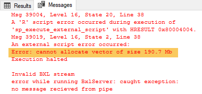
Figure 2: Error Pushing Data
Oh, it looks like we try to push too much data as we see, highlighted in Figure 2, a memory issue. Ok, but this is what the SQLCC is all about - efficiently handling large volumes of data, so let us execute the same code but in the SQLCC (@isCtx bit = 1):
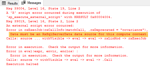
Figure 3: Push and SQLCC Error
Ouch, it seems that to use SQLCC we need to pull data through RxSqlServerData. Never mind, I still want to push large volumes of data, so I change @input_data_1 to do a SELECT TOP(30000000) ... (30 million) from the table instead. When I push my 30 million rows in the local context the execution time is around 17 seconds. What are the timings if we execute the code in Code Snippet 3 with a TOP (30000000) both in the local context as well as SQLCC and compare execution times:
- Local context push (Code Snippet 4 and
@isCtx = 0): ~ 17 seconds. - Local context pull (Code Snippet 3 and
@isCtx = 0): ~ 23 seconds. - SQLCC pull (Code Snippet 3 and
@isCtx = 1): ~ 15 seconds.
That was interesting, the timings between pushing the data in the local context are almost the same as pulling the data in SQLCC, and the push in the local context is much faster than the pull in the same context. What gives?
All we have done so far points to that the difference in performance comes from loading the data, so the question is what the difference is when loading it from the local context compared to the SQLCC, and is SQLCC always faster. Let us start with the last question first; is SQLCC always faster?
To test this change the TOP clause to TOP(50) and execute Code Snippet 4 (pushing the data) and Code Snippet 3 pulling the data both in the local context as well as SQLCC and take note of the timings:
- Local context push (Code Snippet 4 and
@isCtx = 0): ~ 200 ms. - Local context pull (Code Snippet 3 and
@isCtx = 0): ~ 260 ms. - SQLCC pull (Code Snippet 3 and
@isCtx = 1): ~ 1.6 seconds.
That was quite a difference and now, all of a sudden, SQLCC is slowest! Why is that? Let us use Process Monitor to try to figure out why this is the case. However, before we do that let us recap a little bit about the internal workings when we execute SPEES.
Internals
- The host for an external engine is
BxlServer.exe. - When we execute SPEES the SqlSatellite (loaded by the BxlServer) connects to SQL Server over a TCP connection.
- Data is sent over the TCP connection from and to SQL Server.
- The data sent among other things authentication data, script data (the actual external script) as well as the dataset.
The figure below illustrates connections and so forth in a “simple” case where we push data to the SqlSatellite in the local context:
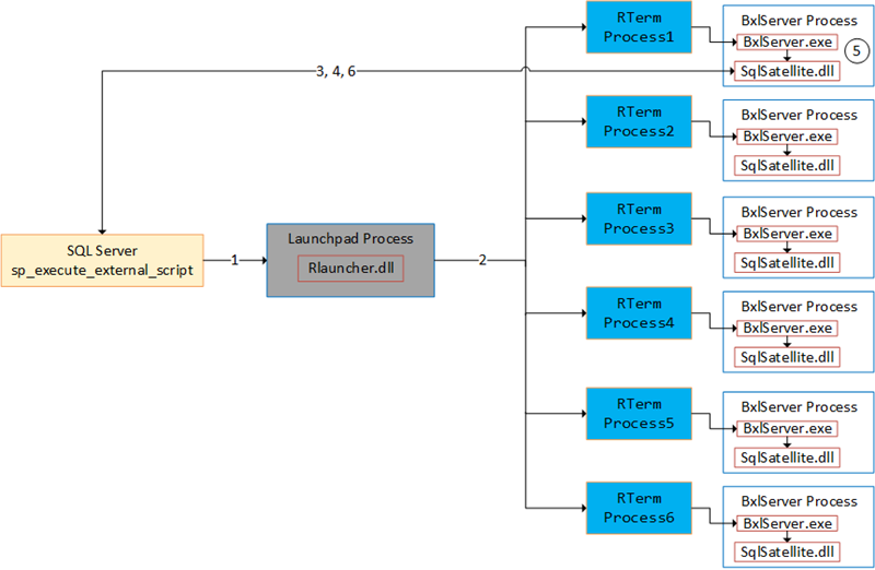
Figure 4: Process Flow
In Figure 4 we see what happens when we execute sp_execute_external_script and the numbers in the figure stands for:
- We call
sp_execute_external_scriptand SQL Server calls into the launchpad service. - The launchpad service creates RTerm processes which in turn creates BxlServer processes. One process becomes the executing process.
- A TCP connection from the SqlSatellite in the executing process gets established.
- SQL server sends input data to the SqlSatellite.
- The
BxlServer.exedoes the processing. - SQL Server receives data back from the SqlSatellite.
The SQL Server R Services series covered in “excruciating” details what data SQL Server sends to the BxlServer. If you want to read up on it I suggest Internals X, XI, XII, XIV and XV.
Investigation using Performance Monitor
To see what happens when we execute our three scenarios (local push, local pull, SQLCC pull) we set up some Process Monitor event filters to capture TCP traffic from SQL Server to the SqlSatellite, where BxlServer.exe is “hosting” the SqlSatellite. The filters we set up are for “Process Name” and “Operation”. We want the process to be BxlServer.exe and the operation “TCP Receive”.
So, run Process Monitor as admin. To set the filter; under the Filter menu click the Filter menu item, and you see the “Process Monitor Filter” dialog. To create the filter we enter the conditions we want to match:
- The Process Name (from the first drop down) should be is (from the second drop-down):
bxlserver.exe. - Operation (first drop-down) is (second dropdown): “TCP Receive”
You add and include the conditions included and added, and at this stage, the filter dialog looks something like so:
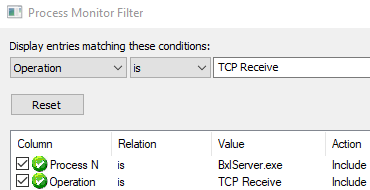
Figure 5: Filters BxlServer
What the filter says is that any “TCP Receive” events for bxlserver.exe should be monitored and displayed. When you have clicked “OK” out of the dialog box, we are ready to test this by executing the code for local context push (Code Snippet 4), local context pull (Code Snippet 3 and @isCtx = 0) and SQLCC pull (Code Snippet 3 and @isCtx = 1). When executing we look at the Process Monitor output, and the output for the local push is like so:
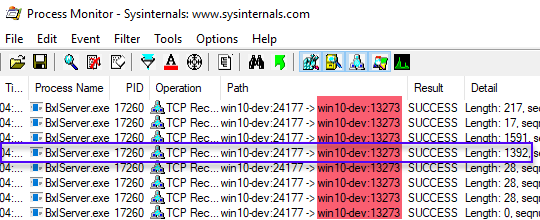
Figure 6: TCP Receive Local Context Push
We see in Figure 6 that the output looks quite “tidy” and by looking at the Path column see a connection between SQL Server and the SqlSatellite on port 13273 (win10-dev:13273). Furthermore, we see:
- There is one
BxlServer.exeprocess with a process id of 17260. - The data the BxlServer receives are what we covered in the SQL Server R Services series.
- The 50 rows we pushed to the BxlServer is the outlined (in blue) row with a length of 1392.
Ok, so onto the local context pull:
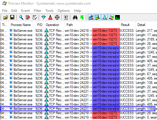
Figure 7: TCP Receive Local Context Pull
Looking at Figure 7 we see that there is quite a difference between when we push the data to the SqlSatellite. First, we see (highlighted in red) the usual connection between SQL Server and the SqlSatellite and how SQL Server sends data (authentication and script) to the SqlSatellite. Then, however, we see data going from SQL Server from a “strange” port: ms-sql-s. That “name” is
IANA’s (Internet Assigned Numbers Authority) definition for SQL Server’s port 1433. As we know, port 1433 is the default port SQL uses for connections and retrieval of data. So it looks like that when we use pull, we connect to SQL Server over the default port and retrieves the data that way. Thinking about it, it makes sense as the connection is an ODBC connection. All the packets received by the SqlSatellite are the regular ODBC data packets. The actual 50 rows of data are in the packet outlined in blue with a length of 1358. As we use ODBC the protocol used to send the data is TDS.
Oh, TDS - that is probably a reason why the local pull is slower than local push, as the local push uses the Binary eXchange Language protocol (BXL) which is very efficient for transferring data. Another reason why the local pull is slower than the local push, even with small datasets, is that for local pull there is much more happening, as we see in Figure 7.
Right, then what about SQLCC pull:
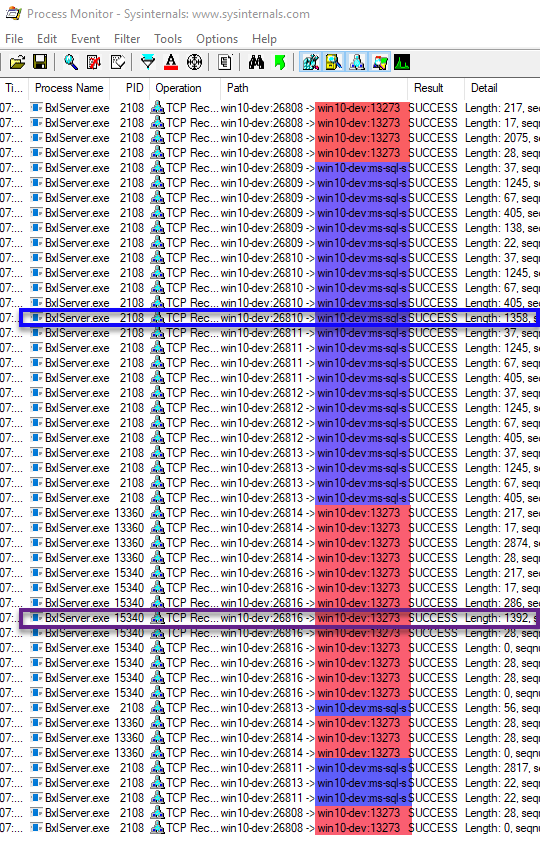
Figure 8: TCP Receive SQLCC Pull
Oh my, that is a lot! As in Figure 7 the sections outlined in red is the connection between SQL Server and the SqlSatellite, and in blue it is the “ODBC” connection. What is noticeable is that there are multiple sections interleaved, as well that there are multiple BxlServer.exe processes involved (process id’s 2108, 13360 and 15340). Well, maybe that is not such a surprise as we spoke about it in
Context - I.
What is more interesting though is that we receive the dataset both via the ODBC connection outlined in blue (length 1358), as well as the way we do it in the local push context, outlined in purple (length 1392)! That means that SQL sends data using both the TDS protocol as well as the BXL protocol.
By seeing the amount of “stuff” happening in Figure 8 we do realise why the SQLCC pull is not as efficient as local push and local pull (1.6 s vs ~200 ms). Having seen all this, we probably ask ourselves why the SQLCC pull was a lot faster (~15 s) than local pull (~23 s) for a big dataset and somewhat faster than the local push (~17 s)?
Let us execute the code in Code Snippet 3 and Code Snippet 4 with TOP (30000000) (30 million) and see what Process Monitor tells us. For local push, we see many packets with a size of 65495 which is the maximum size for BXL data package. When we execute the local pull, we see many TDS packets with a size of 4096 followed by many packages with sizes ranging from ~70,000 up to 2.5 Mb. For me, it looks like the local pull is nowhere as efficient as the local push. Finally, the SQLCC pull shows the same behaviour as local pull with many TDS 4096 packages. However, after the TDS packages follows BXL packages where most have the maximum size of 65495.
NOTE: I do not know why, in the case of SQLCC, data is first loaded via TDS and then BXL. I also do not know why in the case of local pull we see multiple 4096 packages followed by packages with an arbitrary big size. I see if I can find answers to this, in which case update this post (or write a new).
Summary
This post set out to try to find out why SQLCC performs better than local context. I believe we found why this is the reason but not necessarily how it works.
What did we see:
- Local push performs really, really well up until it does not :). It performs well up until you hit memory restrictions.
- Some of the memory issues can be alleviated by using the
@r_rowsPerReadparameter (not shown in this post). - When pushing the data (
@input_data_1) we cannot use SQLCC. - Both local pull as well as SQLCC uses ODBC connections, and the data transfer protocol is TDS.
- When using SQLCC the BXL protocol is also used.
- By the use of BXL we get very efficient processing of data, and that is the reasons we see good performance.
After writing this post, I have quite a few questions which I will try to answer in a future post.
~ Finally
If you have comments, questions etc., please comment on this post or ping me.