A Lap Around SQL Server 2019 Big Data Cluster: Architecture

This post is the second in series about SQL Server 2019 Big Data Cluster based on a presentation I do: A Lap Around SQL Server 2019 Big Data Cluster.

In the first post A Lap Around SQL Server 2019 Big Data Cluster: Background & Technology we looked at - as the title implies - the background of SQL Server 2019 Big Data Cluster, (BDC), and the technology behind it.

In this post, we look at the architecture and components of a BDC.

Before we dive into the architecture, let’s refresh our memories around what we covered in the previous post.

Recap

We are getting more and more data, and the data comes in all types and sizes. We need a system to be able to manage, integrate, and analyze all this data. That’s where SQL Server comes into the picture.

SQL Server has continuously evolved from its very humble beginnings based on Ashton Tate/Sybase code-base to where it is now:

• SQL Server in Linux.
• SQL Server in Containers.
• SQL Server on Kubernetes.

With all the capabilities now in SQL Server, it is the ideal platform to handle big data.

The SQL Server itself is not enough to achieve what we want, so in addition to SQL Server a BDC includes quite a few open-source technologies:

• Apache Spark
• Hadoop File System (HDFS)
• Influx DB
• Graphana
• Kibana
• Elasticsearch
• more …

Oh, and a BDC is not only one SQL server, but quite a few instances. The SQL Server instances are SQL on Linux containers, and the whole BDC are deployed to and runs on Kubernetes (k8s).

We spoke a bit about k8s, and what constitutes a k8s cluster, (nodes, pods, etc.). In the post we tried to illustrate a k8s cluster like so:

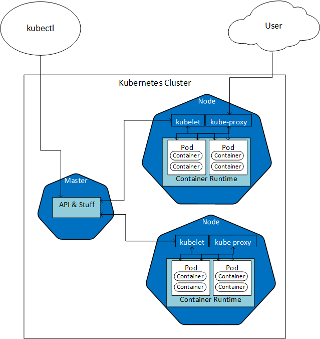
Figure 1: Kubernetes

In Figure 1 we see some of the parts of a two-node Kubernetes cluster, with a Master node. Later in this post, we talk some more about the Master node, and the role it plays.

In the post, we briefly mentioned how we deploy a BDC, and we said we have essentially two options:

• Deploy via Python scripts.
• Deploy using Azure Data Studio.

We looked at how to manage and monitor a BDC, and we spoke about the tools for managing and monitoring:

• kubectl - used to manage the Kubernetes cluster the BDC is deployed to.
• azdata - manage the BDC.

In this post, looking at the architecture, we use the tools above, so ensure you have them installed if you want to follow along.

Architecture

How can we figure out what the architecture looks like? Well, in the A Lap Around SQL Server 2019 Big Data Cluster: Background & Technology post, we discussed k8s pods and how we could get information about the pod by executing some kubectl commands.

So let us go back to the pod we looked at briefly in the last post: master-0, which is the pod containing the SQL Server master instance. We look at that pod to see if we can get some information from it, which will help us in gaining insight into the architecture of a BDC. The code we use looks like so:

1

kubectl get pods master-0 -n sqlbdc-cluster -o JSON

Code Snippet 1: Get Pod Information

In Code Snippet 1 above we see how we use kubectl get pods and we:

• Send in the name of the pod we are interested in,
• Indicate the k8s namespace the pod is in.
• Want the output, -o flag, formatted as JSON.

When we execute the code in Code Snippet 1 we see something like so:

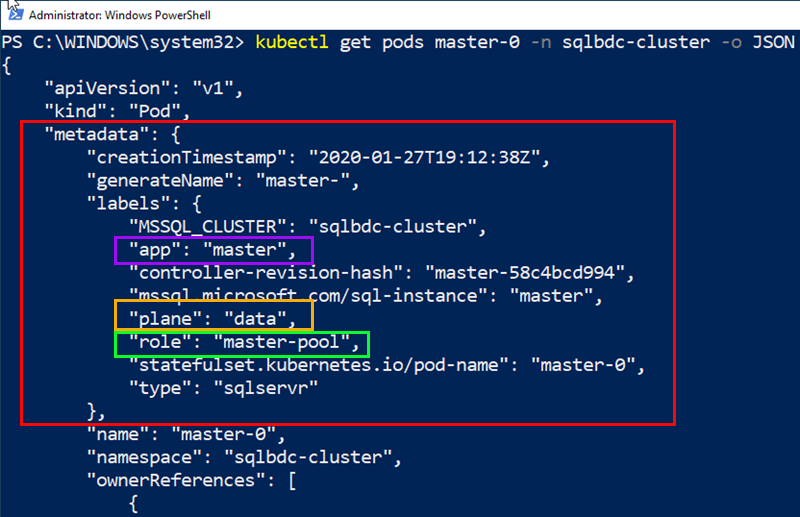
Figure 2: Get Pods

The kubectl get pods master-0 command returns all information about that particular pod, and in Figure 2 we see the first 20 lines or so of the JSON output.

Notice the section outlined in red, the metadata section. This section contains general information about the pod, and if we look closer, we can see three labels outlined in, purple, yellow and green respectively:

• app with a value of master.
• plane with a value of data.
• role with a value of master-pool.

Maybe these labels would give us some insight if we were to look at all pods? Ok, so let’s do that, and we will use some kubectl -o “magic” to get the information we want:

1
2
3
4
5

kubectl get pods -n sqlbdc-cluster \ 
                 -o custom-columns=NAME:.metadata.name, \
                    APP:.metadata.labels.app, \
                    ROLE:.metadata.labels.role,\
                    PLANE:.metadata.labels.plane

Code Snippet 2: Custom Columns

To retrieve the information we want, we use the custom-columns output option. We see in Code Snippet 2 how we say we want four columns back: NAME, APP, ROLE, and PLANE`, and what labels those are, (we talk more about labels below). We then execute:

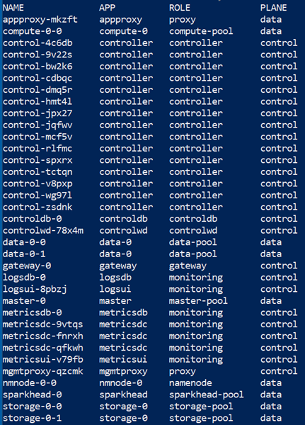
Figure 3: Pods with Custom Output

In Figure 3 we see the result from executing the code in Code Snippet 2 and we see all pods in the sqlbdc-cluster namespace, i.e. all pods in the BDC. From the PLANE column we see how the BDC has two planes, the control plane and the data plane.

Control & Data Plane

Let us make a short diversion here and talk a bit about control and data planes.

In distributed systems/services, we need a way to manage and monitor our services, and that is the role of the control plane. In the previous post we spoke about the master node in a k8s cluster and how we interact with the master node for management of the cluster.

However, k8s has no idea about a SQL Server 2019 Big Data Cluster; in which order pods should be deployed etc. This is where the BDC control plane comes in. It knows about the BDC, so whenever there needs to be an interaction between the Kubernetes cluster and the BDC the k8s master node interacts with the BDC’s control plane. Take a deployment as an example; when deploying to the BDC, the control plane acts as the coordinator and ensures services, etc., are “spun up” in the correct order.

That is, however, not the only thing the control plane does. Remember from my previous post how we briefly discussed monitoring of a BDC and how we said we use Grafana, and Kibana together with the underlying InfluxDB and EleasticSearch as persistent stores. Well, the control plane is also responsible for monitoring, and in Figure 3 you see some examples of this, where there are APP’s related to logs and metrics.

The data plane is what we communicate with when working with the BDC, doing queries etc. - the application traffic. In addition to that, the data plane is also responsible for:

• Routing.
• Load balancing.
• Observability.

Now, knowing a bit about the planes, let us have a look at roles.

role

In Kubernetes, you have the notion of a Role, and that has to do with security: a Role sets permissions within a namespace. The role I refer to here has nothing to do with that. No, a role in this context is a label attributed to a pod in a k8s cluster.

NOTE: In k8s documentation Labels are described as follows: “Labels are key/value pairs that are attached to objects, such as pods. Labels are intended to be used to specify identifying attributes of objects that are meaningful and relevant to users, but do not directly imply semantics to the core system. Labels can be used to organize and to select subsets of objects.”

Seeing the description about Labels above, we can deduce that a role describes the “role” of a Kubernetes component, i.e. what it does or belongs to. With that in mind, we can get some information/insight around the architecture of the BDC from it.

So let us once again look at the pods in the cluster and see what the role labels tell us:

1
2
3

kubectl get pods -n sqlbdc-cluster2 \
                 -o custom-columns=PODNAME:.metadata.name,\
                 ROLE:.metadata.labels.role

Code Snippet 3: Pods & Roles

The code in Code Snippet 3 above is almost the same as in Code Snippet 2, but without the APP and PLANE columns. When we execute, we see:

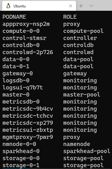
Figure 4: Pods with Custom Output

In Figure 4 we see how the various pods belong to quite few ROLE’s. Some of the ROLE’s we see are familiar, like: controller and monitoring, and we will not talk about them that much more. However, in Figure 4 we also see some ROLEs named xxx-pool. Above we said that the master-0 belonged to a role named master-pool, and we see that in Figure 4 as well.

It turns out that the functionality, (SQL Server Master, Hadoop, etc.), of a BDC, is split into pools.

Pools

When looking at Figure 4 we see that we have different type of pools, and some of them have more than one pod. The pools are:

• compute-pool
• data-pool
• master-pool
• storage-pool

Let us look somewhat more in-depth into the pools above.

Master Pool

From above we see how master-0 belongs to the master-pool. In the last post as well as in this, we have mentioned how the master-0 pod represents the SQL Server master instance, i.e. the “normal” SQL Server where your OLTP databases sit. So, let us see if we can prove that, by looking at what containers the pod has:

1
2
3
4

 kubectl get pods master-0 -n sqlbdc-cluster2 \
                  -o custom-columns=PODNAME:.metadata.name,\
                     ROLE:.metadata.labels.role,\
                     CONTAINERS:.spec.containers[*].name

Code Snippet 4: Master Pod Containers

The code in Code Snippet 4 is almost the same as in Code Snippet 3. The difference is that we also want to see the containers in the pod. When executing, we get:

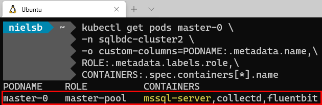
Figure 5: Containers in Master Pod

We see in Figure 5 that the master-0 pod is part of the master-pool, and it consists of three containers. From the previous post we already know about collectd and fluentbit. It is the third container, (first in the list), that is interesting - mssql-server, (highlighted in yellow).

To find out some more about the container we change the code in Code Snippet 4 to the following:

1
2
3
4

 kubectl get pods master-0 -n sqlbdc-cluster2 \
                  -o custom-columns=PODNAME:.metadata.name,\
                     CONTAINERS:.spec.containers[0].name,\
                     IMAGE:.spec.containers[0].image

Code Snippet 5: Container Image

In the code in Code Snippet 5 we see how we retrieve the first container and the first image in the pod. We assume that as the SQL Server container is listed first, (see Figure 5), the container image will also be first. When we execute the code, the result looks like so:

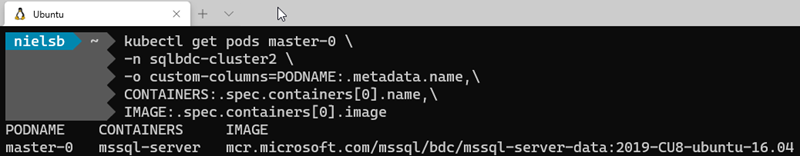
Figure 6: Containers in Master Pod

What we see in Figure 6 is that the SQL Server instance in the master pool is SQL Server 2019 CU8, and it is SQL Server on Linux.

We will see later how there are more SQL Server instances in a BDC, but the master instance is what the user is interacting with. The master instance is also where read-write OLTP or dimensional data is stored, something like so:

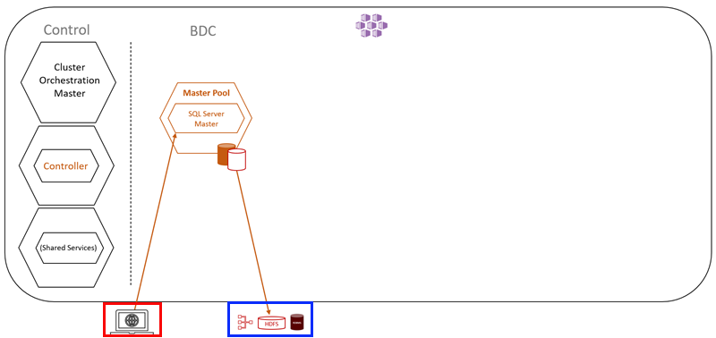
Figure 7: BDC and Master Pool

What Figure 7 shows us is a partial BDC cluster. The left is the control plane as discussed above and then beside it is the master pool with the one SQL Server instance.

At the bottom - outlined in red - we see a screen which illustrates a user and the interaction with the master instance. We also see a picture showing data stores (outlined in blue). What this means is that in SQL Server 2019, (not only BDC), you can query other data stores outside of SQL Server. This is thanks to Data Virtualization and PolyBase.

NOTE: A future post will cover Data Virtualization in SQL Server 2019 BDC.

So, that is the master pool and the SQL Server master instance, what is next?

Compute Pool

In Figure 4 we see how we have one pod belonging to the compute pool, the compute-0-0. Let us find out what containers are in the pod. We use code similar to Code Snippet 4, and when we execute we see:

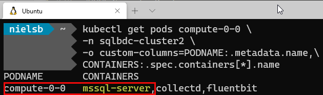
Figure 8: Compute Pool Containers

Hmm, the compute pool pod looks the same as the master pool pod - a SQL Server instance. If we were to look at the container images, we’d see the same as the master instance. So what is this?

As the name implies, the compute pool provides scale-out computational resources for a SQL Server BDC. They are used to offload computational work, or intermediate result sets, from the SQL Server master instance. For you who have worked with PolyBase before it is a fully configured Polybase Scale-Out Group.

The SQL Server instance in the compute pool is - as mentioned before - for computational purposes, not for storing data. The only time there may be data persistence is if it is needed for data shuffling, and in that case, tempdb is used.

If we add the compute pool to what we have in Figure 7 we get something like so:

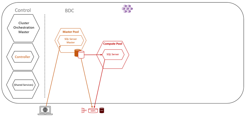
Figure 9: Compute Pool

By looking at Figure 9 we understand that the compute pool is mostly used when accessing external data, and we see more of this as we go along.

Data Pool

When we look at Figure 4 we see we have two pods belonging to the data pool. Let us run the same code as in Figure 8 but replace compute-0-0 with data-0-0 and see what we get:

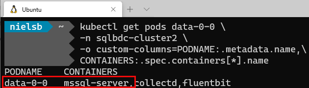
Figure 10: Data Pool & Containers

In Figure 10 we see the same as for the pods in the master and data pools, and if we looked at the second pod it would be the same; one SQL Server instance, together with collectd and fluentbit. So the only difference between the data pool and the other pools is that we have two SQL Server pods in the data pool. Building on the architectural diagram, it looks like so:

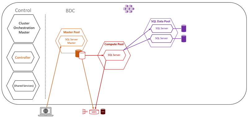
Figure 11: Data Pool

We see the data pool in Figure 11, and how it has the two SQL Server instances mentioned above. The reason it has two is that the data pool acts as a persisting and caching layer of external data. The data pool allows for performance querying of cached data against external data sources and offloading of work.

You ingest data into the data pool using either T-SQL queries or from Spark jobs. When you ingest data into the pool, the data is distributed into shards and stored across all SQL Server instances in the pool.

NOTE: The data pool is append only, you cannot edit data in the pool.

At the beginning of the post, we mentioned Apache Spark and Hadoop, but so far we have only seen SQL Server “stuff”. Where is Hadoop?

Storage Pool

In the previous paragraph, we asked where Hadoop comes into the picture, and the answer to that is the storage pool. Let us have a look at one of the pods in the storage pool and see what information we get. We use the same code as for the other pods, and when we execute, we see:

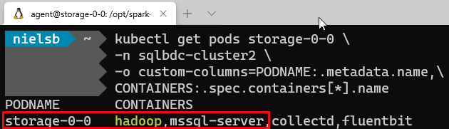
Figure 12: Storage Pool & Containers

That is interesting! In Figure 12 we see the “usual suspects”; mssql-server, collectd, and fluentbit - but we also see a container we haven’t seen before: hadoop.

We have two pods in the storage pool, and the hadoop container in each pod forms part of a Hadoop cluster. The Hadoop container provides persistent storage for unstructured and semi-structured data. Data files, such as Parquet or delimited text, can be stored in the storage pool. Not only is the Hadoop File System, (HDFS), within the container but also Apache Spark:

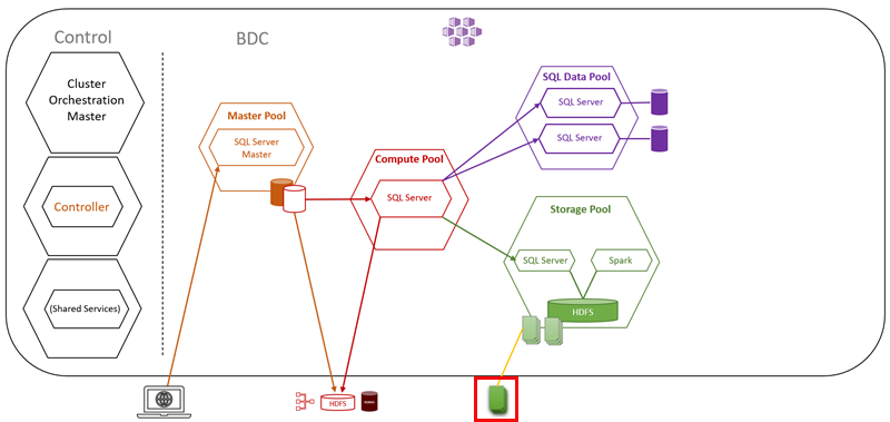
Figure 13: Storage Pool

We have added to our architectural diagram the storage pool cluster as in Figure 13, and at the bottom of the picture, outlined in red, something that looks like files. That represents the ability to mount external HDFS data sources into the storage pool cluster. You access the data via the SQL Server master instance, and PolyBase external tables or you can use the Apache Knox Gateway which sits in the Hadoop name-node: nmnode-0-0, which you see in Figure 4.

You may ask why we have SQL Server instances in the storage pool pods? The Big Data Cluster uses the SQL Servers to optimize the access of the data stored in the HDFS Data Nodes.

We have now looked at the various pools we listed at the beginning of this post, and we should have a relatively good grasp of the architecture of a SQL Server 2019 Big Data Cluster.

Applications

However, there is one thing more to look at. If we look at Figure 4 we see at the very top a pod named appproxy-nsp2m, and its role is proxy. What is this? Well, let us run the same code we have done so many times before and see that containers this pod has:

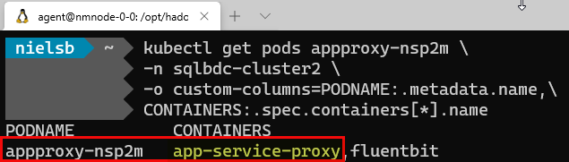
Figure 14: Application Proxy

In Figure 14 we see that the appproxy-nsp2m has a container named app-service-proxy. This container is used, amongst other things, to enable applications to be deployed to a BDC.

Application Pool

The reason for deploying applications to the BDC is so the applications can benefit from the computational power of the cluster and can access the data that is available on the cluster. Supported runtimes are:

• R
• Python
• SSIS
• MLeap

When we deploy an application to a BDC, it is deployed into the Application Pool:

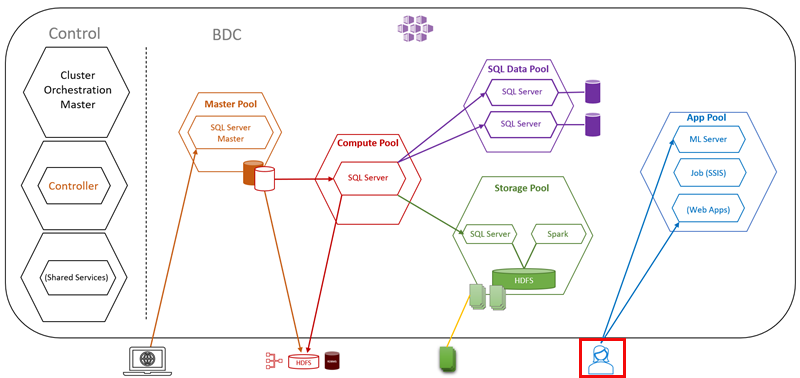
Figure 15: Application Proxy

What we see in Figure 15 is an example of the application pool where we have a user, outlined in red, interacting with the applications in the pool.

Summary

This is the second post in a series about SQL Server 2019 Big Data Cluster. In the first post: A Lap Around SQL Server 2019 Big Data Cluster: Background & Technology we looked at the reason why SQL Server 2019 Big Data Cluster came about and the tech behind it.

In this post, we looked at the architecture of the BDC. We discussed in this post about:

• Master Pool: the master instance of SQL Server, which also acts as an entry point into the BDC.
• Compute Pool: provides scale-out computational resources for a SQL Server big data cluster.
• Data Pool: persistence and caching layer for external data.
• Storage Pool: provides persistent storage for unstructured and semi-structured data.
• Application Pool: hosts applications running inside the BDC.

In future posts, we will look at data virtualization, and how the various pools work.

~ Finally

If you have comments, questions etc., please comment on this post or ping me.

• ← Previous Post
• Next Post →