One Billion Row Challenge & Azure Data Explorer

On January 1st (that’s dedication - New Year’s Day), 2024 Gunnar Morling published on his blog the One Billion Row Challenge. The challenge is to load and aggregate one billion rows using Java. The challenge took on a life of its own, and there are now several implementations of the challenge in different languages, including databases ( Robin, Hubert, Francesco, among others). The data to aggregate is a list of temperature readings from weather stations.

I thought It would be fun to do the challenge using Azure Data Explorer (ADX) since I like ADX and have written blog posts about it. ADX is a fast, scalable, and highly available data analytics service. It is optimized for data exploration over large data volumes. ADX is a columnar store that uses a query language called Kusto Query Language (KQL). It is a fully managed service, and it is part of the Azure platform.

So, in this blog post, you’ll see what I did to load and aggregate one billion rows. Spoiler alert: certain things didn’t work out as I had hoped, but that could be due to me being more rusty with ADX than anything else.

Caveat

Before we get started a couple of caveats:

• I’m not going to do a performance analysis of ADX. I’m going to show you how I loaded and aggregated one billion rows using ADX, not comparing ADX to other databases, languages, etc.
• As we are aggregating data, I see the workload as an analytical workload, where data would - most likely - be continuously streamed into ADX. So therefore I am not looking at the load time of the data, but rather the time it takes to aggregate it.

I mentioned the above about loading the data because the original version of the challenge was the time it took to load and aggregate the data.

Pre-Reqs

This section is here to list what you need if you want to follow along:

• An Azure account. If you don’t have an Azure subscription, sign up for a free account.
• An ADX cluster and database. To set up an ADX cluster and a database, look here: Quickstart: Create an Azure Data Explorer cluster and database. You can name the database as you like. My database is called sensorreadings. Please note that there may be a cost associated with the ADX cluster, so be sure to tear it down when you are done.

You may have seen how ADX offers free clusters. A free cluster allows you to explore the platform’s features, experiment with data analytics queries, and develop proofs of concept without incurring any cost. I tried to use a free cluster for this blog post, but I ran into a couple of issues, so I am using my “tried and tested” cluster from previous blog posts about ADX instead. If you follow along, you can try using a free cluster, but I cannot guarantee it will work.

After all this, the assumption is that you now have a running ADX cluster.

Java

You also need Java, and specifically Java 21. I did the challange on my Windows box so I used Chocolatey to install Java:

1

$ choco install openjdk --version=21.0.1

Code Snippet 1: Install Java

After running the code in Code Snippet 1, I had to “fix up” my PATH environment variable, as it was pointing to the wrong version of Java. Having fixed that and restarted my terminal, I ran java -version and got the correct version. Success!

Generating the Data

Where do you get the one billion rows from to load into ADX? Well, you generate it. Gunnar supplies a Java program (hence the Java requirement above) that generates the data. Fork Gunnar’s repo and clone it locally.

After having cloned the repo, you build the Java program using Maven:

1

$ ./mvnw clean verify

Code Snippet 2: Build the Java App

Having built the application as in Code Snippet 2, it is time to generate the data. Gunnar’s Java program takes a single argument: the number of rows to generate:

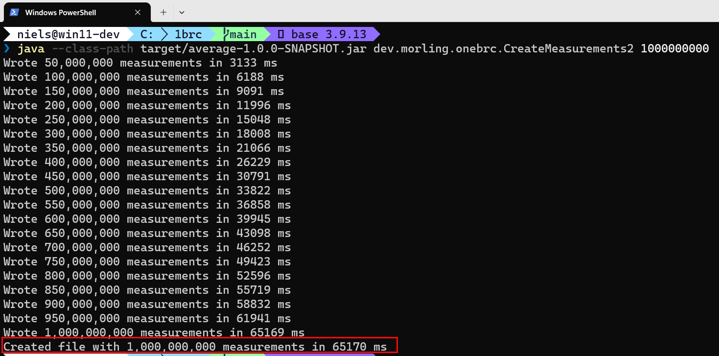
Figure 1: Generate the Data

In Figure 1 you see how I generated one billion rows. I did not do it as per Gunnar’s instructions, executing a .sh file as I had some issues on my Windows box running the command. Instead, I directly executed the Java program the .sh file pointed to. The result is the same: I generated a file with one billion records.

NOTE: Be aware that the file generated will be large, around 13Gb. So make sure you have enough space on your disk.

Generating the records took ~65 seconds on my machine (as in Figure 1) and created the file measurements2.txt. The file is created in the root folder of the cloned repo.

The Data

The data generated is the name of the weather station and the temperature reading, semi-colon delimited:

1
2
3
4
5

Mogadishu;29.1
Fresno;24.1
Dakar;18.7
Mombasa;35.7
Vienna;5.1

Code Snippet 3: Sample of the Data

You see in Code Snippet 3 a sample of the data. The station name is a string, and the temperature is a double.

You should now be ready to load the data into ADX. However, the generated file is 13Gb and from a performance perspective, it is not feasible to load the file as is. So, you need to split the file into smaller files.

Split the Data

I use the split command to split the file into smaller files. However, the split command is a Linux command, and I am on Windows; what to do? I have two options:

• Use Windows Subsystem for Linux (WSL).
• Use Git-Bash.

I have both installed on my machine, and I decided to use WSL. I ran the following:

1

$ split -l 50000000 measurements2.txt

Code Snippet 4: Split the Data

The command in Code Snippet 4 splits the file into smaller files, each containing 50 million rows.

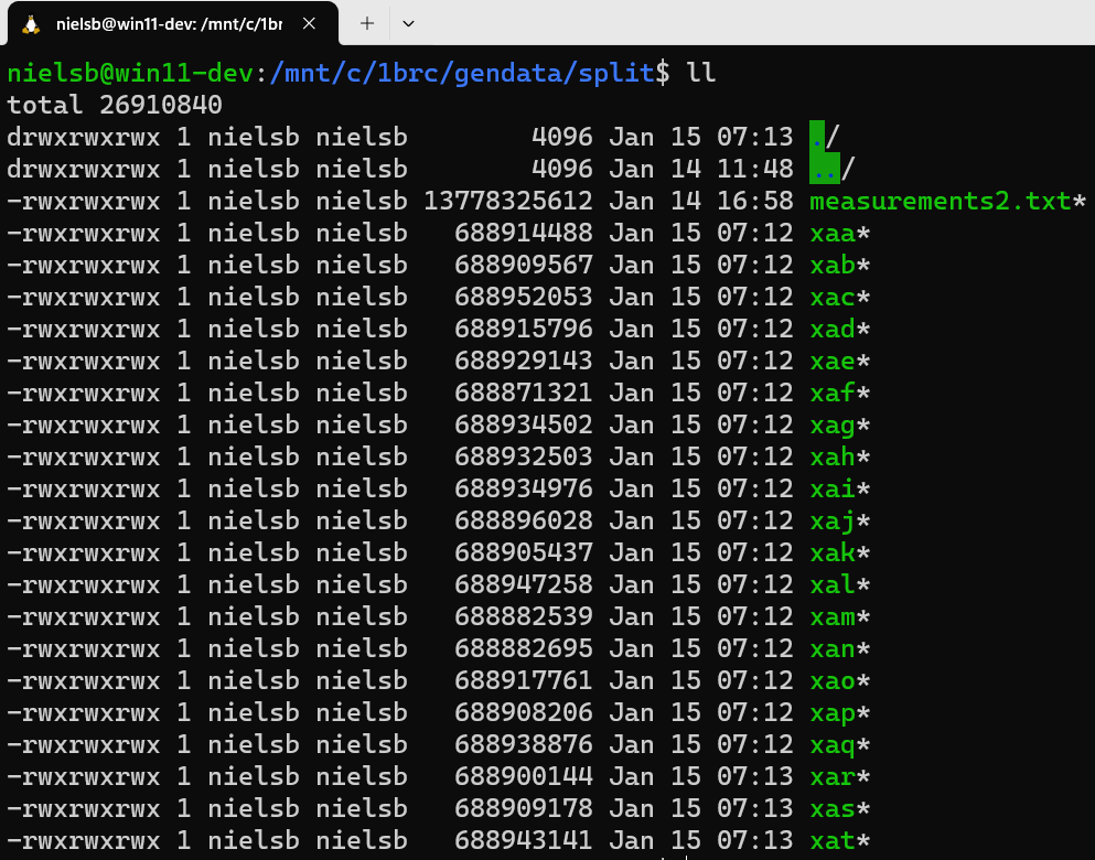
Figure 2: Split Files

In Figure 2, you see the result of running the command in Code Snippet 4. The files created when running the command are named xaa, xab, xac, etc., and are created in the same folder as the original file. As the timestamp column in Figure 2 shows, the command took ~1 minute to run (started at 07:12 and ended at 07:13).

Initially, when I played around with investigated loading the data into ADX, I had some problems which I attributed to the files not having an extension. So, I ran a PowerShell command to add the .txt extension to the files:

1

$ Get-ChildItem -exclude '*.doc','*.txt' | Where-Object {!$_.PsIsContainer} | Rename-Item -newname {$_.name + ".txt"}

Code Snippet 5: Add Extension to Files

After running the command in Code Snippet 5, the files had the .txt extension, and I am getting closer to loading the files.

Loading the Data

A while back, I wrote a series of posts about iGaming leaderboards and ADX, Develop a Real-Time Leaderboard Using Kafka and Azure Data Explorer. In the post Develop a Real-Time Leaderboard Using Kafka and Azure Data Explorer - II, I discussed how to batch-ingest data from local files into ADX.

NOTE: Yeah, I know, I know - I still need to finish that series. I will, I promise. I just got sidetracked by other things.

In the post mentioned above, I used the ADX Ingestion wizard to ingest the data from the files into ADX. However, with the amount of data, 20 files weighing in at ~670 Mb each, I decided to use the LightIngest tool instead. LightIngest is a command-line utility for ad-hoc data ingestion into ADX. The utility can ingest data from various sources, including files from a local folder, and the docs says: …most useful when you want to ingest a large amount of data, …. This led me to believe that Light Ingest would be a good fit.

Well, it didn’t go to plan as I got the weirdest errors no matter what I did. I spent several hours trying to figure out what was wrong, to no avail. So, I decided to use Azure Blob Store instead. First, upload the files to the blob store, then ingest the data into ADX. I started with creating a storage account and a container in the storage account. I then uploaded the files to the container. That worked fine:

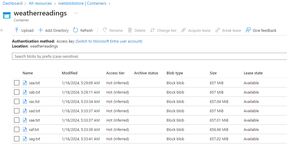
Figure 3: Azure Blob Store

Having the data in the blob store as in Figure 3, I can now ingest it into ADX. My idea was to use the same approach as in the post above - using the Ingestion wizard. Or rather, the replacement for the Ingestion wizard:

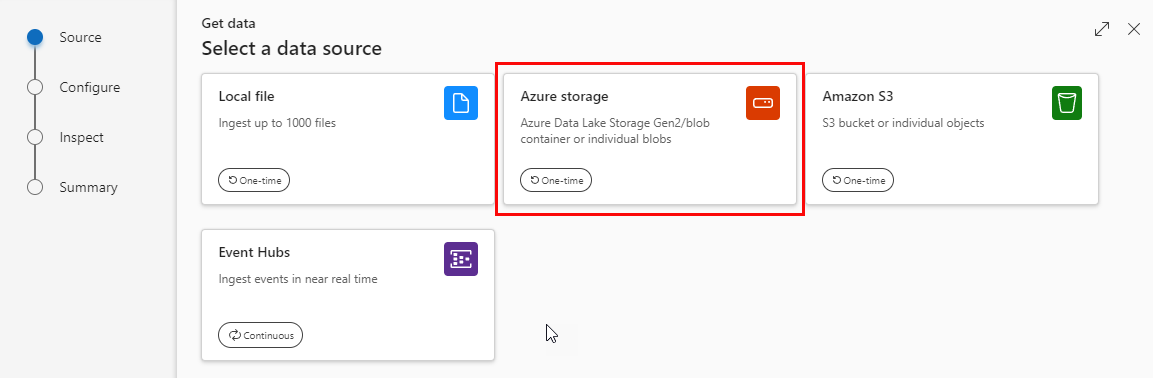
Figure 4: Get Data - Select Data Source

You get to the Select a data source dialog in Figure 4 by right-clicking on your database and selecting Get data.

I’ll get to what to do to set up and ingest the data in a minute, as before you can ingest, you need to prep your database a bit.

Ingestion Mapping

When ingesting data into ADX, you need to specify to where and how the data should be ingested:

• Database
• Table
• How the data in, in this case, file(s) should map to the table.

ADX can handle different file formats, like CSV, JSON, Parquet, etc. In this case, the file is a text file, and the data is semi-colon delimited. That is a problem as ADX does not support semi-colon delimited files (at least, I have yet to find a way to ingest semi-colon delimited files directly).

NOTE: It is quite disappointing that ADX only supports comma-delimited files. I expected to be able to indicate what delimiter to use, but no.

So, I need to ingest the data into a one-column table and then, somehow, parse the semi-colon delimited data in the table into another table. I’ll get back to that later.

Creating the Table(s)

Let’s create the tables first:

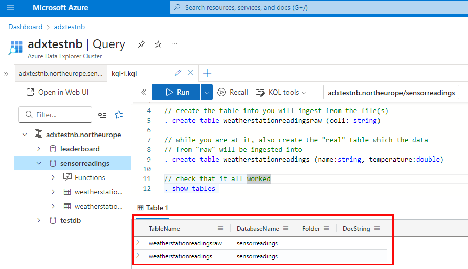
Figure 5: Create Tables

In Figure 5, you see how I, in my cluster’s Query editor, not only created the table I will insert the data from the files but also the table the parsed data will be inserted into. The table names are weatherstationreadingsraw and weatherstationreadings. The table weatherstationreadingsraw is where the data from the files will be inserted, and weatherstationreadings is the table into which the parsed data will be inserted.

You also see in Figure 5 how I, as last statement, ensure that it has worked ok by executing . show tables. As you see - outlined in red - all is OK.

Cool, so now you have the tables, and theoretically, you can now ingest the data from the files into the table weatherstationreadingsraw. Having ingested the data into the table weatherstationreadingsraw, you can then parse the data into the table weatherstationreadings using some smart KQL. However, there is a better way, where the ingestion from the files in the blob store and the parsing into the other table is done in one go.

Update Policy

An ADX update policy instructs ADX to automatically ingest data into a target table whenever new data is inserted into the source table. During the ingestion into the target table, the data can be queried/manipulated. The query/manipulation of the data ingested into the source table is done using a function. The policy then links the source table, the target table, and the function.

Let’s start with the function:

1
2
3
4
5
6
7

// create the function which will parse the data coming into the source table
. create function 
  SplitColumn() { 
    weatherstationreadingsraw 
    | parse col1 with name:string ';' temp:double
    | project-away col1
  }

Code Snippet 6: Create Function

The function in Code Snippet 6 uses the KQL parse operator to split the column col1 into name and temp columns. It splits it based on the semi-colon ';' in the column. The function then excludes the column col1 from the target table using the project-away operator, as it is no longer needed.

When you have created the function, you create the update policy:

1
2
3
4
5
6
7
8

.alter table weatherstationreadings policy update 
@'['
    '{ "IsEnabled": true,' 
    '   "Source": "weatherstationreadingsraw",' 
    '   "Query": "SplitColumn()",' 
    '   "IsTransactional": true,' 
    '   "PropagateIngestionProperties": false}'
 ']'

Code Snippet 7: Create Update Policy

You see in Code Snippet 7 how you create the update policy by altering the target table. The update policy instructs ADX to automatically ingest data into the target table (weatherstationreadings) whenever new data is inserted into the source table (weatherstationreadingsraw). The data is ingested using the function SplitColumn(). The update policy is transactional, meaning that if the ingestion into the target table fails, the data is not inserted into the source table.

NOTE: You can read more about update policies here.

Now, you are ready to ingest the data from the files into the source table.

Ingest the Data

As I mentioned before, I initially tried to ingest the data from the files being local to my computer. That didn’t work, so I uploaded the files to Azure Blob Store and now want to ingest them from there.

So, as in Figure 4 I selected Azure Blob Storage as the data source (after having right-clicked on the database and selected Get data). I then choose the table I want to insert the data into:

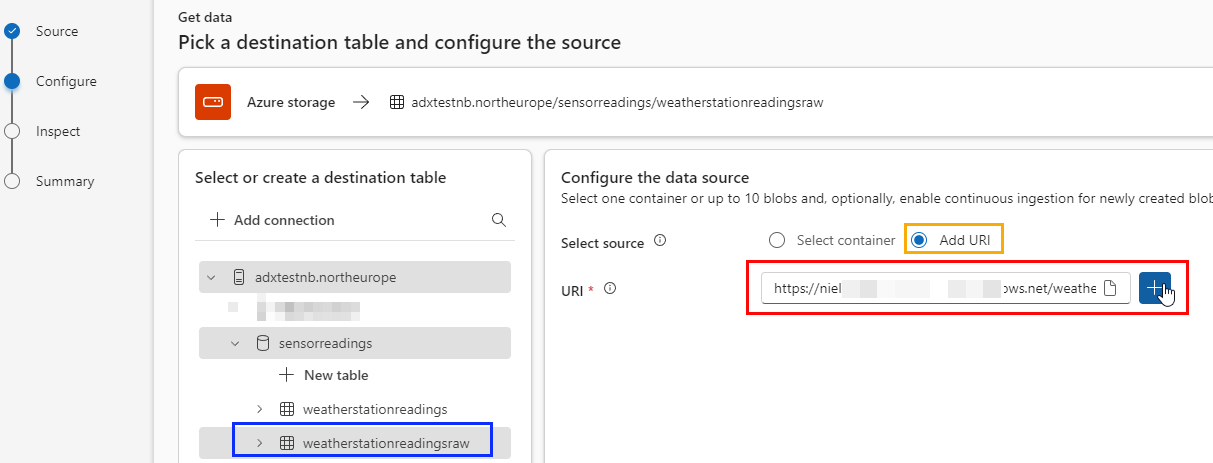
Figure 6: Configure Source

After choosing the weatherstationreadingsraw table to ingest the data into I configure the data source as in Figure 6. You see how I have chosen to add the data from a URI (outlined in yellow) and added my blob store’s container URI (highlighted in red). Having entered the URI, I click on the plus sign and then Next:

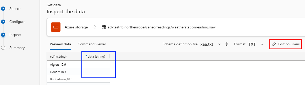
Figure 7: Inspect Data

When clicking Next in the Configure Source dialog, I get to the Inspect the data dialog in Figure 7. The dialog chooses one file in the container as the schema definition file and you see in the figure that it is the file xaa.txt. The dialog correctly picks up the file format as TXT. However, as ADX doesn’t understand other delimiters than commas, it gets confused and believes the file contains two columns, col1 and data. This means I have to click Edit columns:

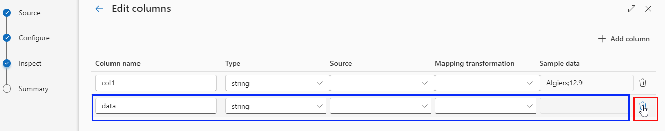
Figure 8: Edit Columns

You see in Figure 8 the Edit columns dialog. The dialog correctly shows the first column (col1), but I must delete the second column outlined in blue. I delete the column by clicking on the “trash can” icon outlined in red, and then I click Next:

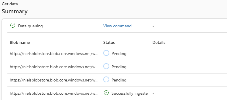
Figure 9: Get Data Summary

In Figure 9 you see the Summary dialog. The dialog has two parts: the Data preparation (partially hidden in Figure 9) and the Blob name. In the Data preparation, you see the commands created for ingesting the data. In the Blob name you see the names of the individual blobs and their ingestion status. Running the ingestion will take a while, so if you do it, I suggest you take a break and go for a walk or something.

NOTE: Another slight disappointment is how long the ingestion took. It took well over an hour to ingest the data. I would have expected it to be faster.

Eventually, all the blobs will be ingested, and you will see a status of Successfully ingested for all blobs, and at the top of the Summary dialog, you see:

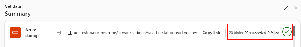
Figure 10: Ingestion Complete

As you see in Figure 10, outlined in red, 20 blobs were targeted for ingestion and 20 blobs were successfully ingested. Yay!

To further confirm things are good, you can execute the following query:

1
2

weatherstationreadings 
| count

Code Snippet 8: Count Rows

The query in Code Snippet 8 counts the number of rows in the table weatherstationreadings. You should see a result of 1,000,000,000 rows!

Aggregating the Data

Now that you have the data in the table weatherstationreadings, it is time to aggregate it according to the challenge. The challenge is aggregating the data by station and calculating each station’s average, minimum and maximum temperature.

When you aggregate data in ADX, you use KQL’s summarize operator:

1
2

T
| summarize output_column = aggregation_function(input_column) by grouping_column

Code Snippet 9: Summarize

In Code Snippet 9, you see the syntax for the summarize operator. The operator takes an input column from the table T and an aggregation function and groups the data by one or more grouping columns. The aggregation result is a new column(s), which can be named (output_column). If not named, the column(s) will be named after the aggregation function plus the source column name (aggregation_function_input_column).

So, to aggregate the data in the table weatherstationreadings you use the following query:

1
2
3
4

weatherstationreadings
| summarize min_temp = min(temperature), 
            avg_temp = avg(temperature), 
            max_temp = max(temperature) by name

Code Snippet 10: Aggregate Data

The query in Code Snippet 10 aggregates the data in the table weatherstationreadings by station name. The aggregation functions used are min, avg and max; the result is three columns: min_temp, avg_temp and max_temp, plus the name column.

When executing the query in Code Snippet 9, you should see a result similar to the following:

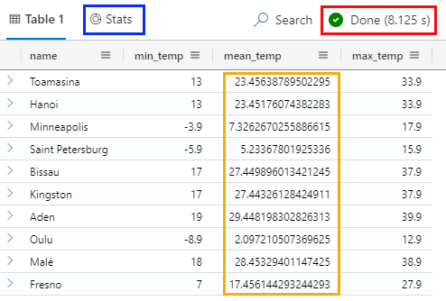
Figure 11: Aggregate Data

There are a couple of things to note in Figure 11:

• The query took ~8.1 seconds to execute (outlined in red). Good for aggregating one billion rows.
• You can get a more detailed view of the stats of the query by clicking on the Stats button (outlined in blue).
• The values in the mean_temp column have a lot of decimals (outlined in yellow).
• The result is not ordered by station name.

Let’s try to fix the last two points:

1
2
3
4
5

weatherstationreadings
| summarize min_temp = round(min(temperature), 1), 
            avg_temp = round(avg(temperature), 1), 
            max_temp = round(max(temperature), 1) by name
| order by name asc

Code Snippet 11: Aggregate Data - Round and Order

In Code Snippet 11, you see how I use the round() operator to round the columns to one decimal and order the result by station name. The result of executing the query in Code Snippet 11 is:

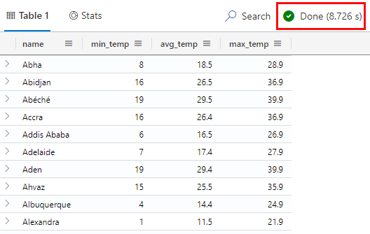
Figure 12: Aggregate Data - Round and Order

In Figure 12, you see the result of executing the query in Code Snippet 11. The avg_temp column now has one decimal, and the result is ordered by station name. The query took ~8.7 seconds to execute (outlined in red). This is a smidge longer than the previous query, but not by much.

What is interesting if you look at Figure 12 is that I did the round() operation against the min_temp column, and I would expect to see the likes of 8.0, 16.0, etc., where the result has no fractional value. As you can see, that is not the case. I tried all sorts of things, casting to double, etc., but no luck. The one thing that worked was to cast the column to a string: min_temp = tostring(round(min(temperature), 1)),. However, that feels ugly. If a numeric value decimal, etc., has no fractional part, you can’t show with a 0 as the fractional part unless you cast it to a string. If you know of a better way, please let me know.

Formatting the Result

The challenge added a further “twist”. The aggregation result should be output as a string in a specific format: station name=min/mean/max, name=min/mean/max, etc. Something like so:

1

"{Mogadishu=29.1/29.1/29.1, Fresno=24.1/24.1/24.1, Dakar=18.7/18.7/18.7, Mombasa=35.7/35.7/35.7, Vienna=5.1/5.1/5.1, ...}"

Code Snippet 12: Formatted Result - I

To achieve the desired result as in Code Snippet 12, I use a couple of cool KQL operators:

1
2
3
4
5
6
7
8

let T = 
weatherstationreadings
| summarize min_temp = tostring(round(min(temperature), 1)), 
            avg_temp = round(avg(temperature), 1), 
            max_temp = max(temperature) by name
| order by name asc;
T
| summarize result = make_list(strcat(name, '=', min_temp, '/', avg_temp, '/', max_temp))

Code Snippet 13: Format the Result - I

You see in Code Snippet 13 how I started by using the let statement to create a CTE/temporary table T containing the aggregated data. I use T to concatenate the columns name, min_temp, avg_temp and max_temp into a string using the strcat() operator. Having each row concatenated, I finally apply the make_list() function, which creates a dynamic array.

That worked fine, but I wanted to know whether I could do it in one go. It turns out I could:

1
2
3
4
5
6

weatherstationreadings
| summarize min_temp = tostring(round(min(temperature), 1)), 
            avg_temp = round(avg(temperature), 1), 
            max_temp = max(temperature) by name
| order by name asc            
| summarize result = make_list(strcat(name, '=', min_temp, '/', avg_temp, '/', max_temp))

Code Snippet 14: Format the Result - II

Pretty cool how I can have multiple summarize operators in a query. The result of executing the query in Code Snippet 14 is:

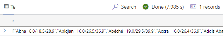
Figure 13: Final Result

As you see in Figure 13, the result pretty much looks as it should. Awesome!!

Summary

In this post, you have seen how I loaded one billion rows into ADX. I did it by uploading the data to Azure Blob Store and then ingesting it from there.

Having the data in Azure Blob Store, I used ADX’s built-in functionality to ingest data from the source. Since ADX does not understand semi-colon as a delimiter I had to ingest the data into a one-column table and then parse the data into another table. I did that by using an update policy.

I then aggregated the data using the summarize operator and respective aggregation functions. Finally, I formatted the result using multiple summarize and the make_list() function.

Disappointments

As much as I like ADX and KQL, there were a couple of things that disappointed me:

• LightIngest did not work as expected (this could have been a me thing). It seemed to be due to the number of files and their size, but as I said, I could be doing something stupid.
• The ingestion of the data took a long time. I would have expected it to be faster.
• It looks like ADX doesn’t support any delimiters other than commas. I expected to be able to indicate what delimiter to use, but no.
• It seems that if a decimal value has no fractional part, you can’t show with a 0 as the fractional part, unless you cast it to a string.

Cool Things

There were also a couple of cool things:

• KQL’s built-in functions to do “stuff” with the data, like make_list(), parse etc.
• The ability to have multiple summarize operators in a query. That is uber cool!

~ Finally

If you have comments, questions etc., please comment on this post or [ping][ma] me.

• ← Previous Post
• Next Post →